Tying is not always simple

Tying in most useful cases requires complex function $g$.

• Simple models → High bias error
• Complex models → Variance error plus harder to train

Ad hoc tying requires human tailored configuration and is hardly considered learning.

XOR problem

We cannot always represent complicate functions with simple models.
For example, the XOR function, only two layers will not work! (Linearly inseparable.)

An idea to go deeper

A deeper model can represent XOR. The first layer map the inputs into a linearly separable space.

Training in deep models

Search techniques: Hessian free, BFGS, simple gradient descent.
All search techniques require forward-propagation of input values.
Deeper models have prices: propagation of activation signals through untrained higher levels create arbitrary beliefs for top levels. Most of the time, higher layers are trained with arbitrary data and get stuck at some local minima.
It is better to train layer-by-layer, not all layers at once.

Deep architecture

We can do unsupervised learning layer-by-layer to produce hierarchy of feature detectors.
The benefit of going deeper is to acquire more information from different spaces and times.
Higher, deeper layer will represent more complex patterns on top of features from lower layers.
Each layer extracts simple patterns from the training data, which are shared among many high level features. This in turn reduces the number of model parameters.

Visual cortex has some depth

The lowest level detects edges while higher levels capture more complex features.

Deeper implies compact information

When inputs are categorized, the group variance indicates the true underlying information. That is deep models with unsupervised learning tries to reduce redundancy in the data.
At the top most level, data are compact.

Compact implies generalized

Redundancy (correlation) tampers the true distance between representations of two data. Learning tries to remove it.
Once redundancy has all been removed. We cannot predict any part of the fully compressed data. They are the underlying information within the data.
The most compact representation is fully generalized representation.

Compact representation

Generalization

• Perceptive generalization: the ability to recognize the same parts within similar data. This also means the recognition of the true distance between data.
• Adaptive generalization: adaptive responses to given inputs. This requires tying of the output modules to the compact internal representation which presents the true factors that govern the causes of actions. The most compact representation is to where any module converges without knowledge of one another.

World's information space

Objects within the same space or time proximity tend to relate: causality or mere correlation. Deep learning can map two seemingly unrelated inputs into the same group if they appear together in the same space-time vicinity.
If the brain can form bases for this space, the brain is generalized.

Nature of the brain

• The brain tries to remap perceptions into space-time related space.
• It must be able to reproduce the learned information. (This is aspect of memorization.)

Killing two birds with a stone

If our brains manage to form the generalized information space, we also get a relatively good generative model.
Information is in fact randomness. This conforms with the native activation pattern of cells at the intrinsic level.

Neural tying

Linear tying rule between a pair of neuron layers, say $\textbf{h}$ and $\textbf{v}$:

Capture and tie

Before unsupervised training, the activation pattern of internal layer $\textbf{h}$ is not defined.
We randomly generate $\textbf{h}$ from current $W$ and $\textbf{v}$ and tie them together.
If $W$ captures some patterns in $\textbf{v}$, $\textbf{h}$ will be activated. And the stronger the $\textbf{h}$ is, the further the relation is enhanced.
Initial weights should not be all zeroes. (Symmetry breaking.)
This is stochastic pattern grouping!

Expectation-Maximization

Originally people view Expectation-Maximization (EM) as an algorithm used to model $\log P(\textbf{v})$:
$ \begin{align} \log P(\textbf{v}) =& \sum_{\textbf{h}} P(\textbf{h}|\textbf{v}) \left( \log P(\textbf{v}|\textbf{h}) + \log P(\textbf{h}) - \log P(\textbf{h}|\textbf{v}) \right) \end{align} $
But maximizing exact $\log P(\textbf{v})$ requires the knowledge of posterior $P(\textbf{h}|\textbf{v})$ which is hard to compute. (Explaining away.)
So EM updates the lowerbound instead:
$ \begin{align} \log P(\textbf{v}) \geq& \sum_{\textbf{h}} Q(\textbf{h}|\textbf{v}) \left( \log P(\textbf{v}|\textbf{h}) + \log P(\textbf{h}) - \log Q(\textbf{h}|\textbf{v}) \right) \end{align} $
There is another interpretation...

EM finds compact representation

The mechanism we use to categorize data leads to compact representation.
This in turn improves the lowerbound of generative model.
Which is why killing two birds by one stone.

Proof sketch

$ \begin{align} \log P(\textbf{v}) \geq& \sum_{\textbf{h}} Q(\textbf{h}|\textbf{v}) \log P(\textbf{v}|\textbf{h}) - \text{KL}( Q(\textbf{h}|\textbf{v}) || P(\textbf{h}) ) \end{align} $
The lowerbound consists of two terms: information preservation and posterior-prior divergence.
The second term is minimized when the data representation $Q(\textbf{h}|\textbf{v})$ matches the prior $P(\textbf{h})$.
The brain favors sparse prior distribution. (We shall see later on.)

Proof sketch

Sparsity can be derived from independent component analysis, which also implies uncorrelated bases per se.
If we run capture and tie, at convergence data that are correlated will be tied and merged together. Only uncorrelated, distinct patterns will stand out.

Proof sketch

Consider the original form of the hebbian rule: $\begin{align} \nabla \textbf{W} = \sum \textbf{h}\textbf{v}^\intercal = \sum \textbf{W}\textbf{v}\textbf{v}^\intercal = \textbf{W}\textbf{C} \end{align}$
$\textbf{C}$ is the covariance of matrix of the data.
The solution to this equation given the constraint that each column vector has a fixed length is the eigenvectors of $\textbf{C}$.

Variants of EM

Dimensionality reduction techniques.

• PCA
• Factor analysis
• K-means
• Gaussian mixture

Contrastive divergence

This technique drives the popularity in deep learning since 2006 by Geoffrey Hinton.
The normalization factor is the stationary distribution of the bipartite network (RBM).
We want the stationary distribution to match the input distribution activate. Therefore, the update gradient is the difference between input and stationary distribution. $\nabla W = \sum_{\textbf{h}} P(\textbf{h}|\textbf{v}) (\textbf{h}.\textbf{v}^\intercal) - \sum_{\textbf{k},\textbf{u}} P(\textbf{k},\textbf{u}) (\textbf{k}.\textbf{u}^\intercal)$

Contrastive divergence (2)

We use blocked Gibb's sampling to sample the stationary distribution.

Contrastive divergence (3)

Unlike conventional EM, CD provides training procedure for the true generative model $\max \log P(\textbf{v})$ (not the lowerbound, Yee-Whye Teh). It has been proposed to solve the problem of finding the true posterior; for CD-trained RBMs: $Q(\textbf{h}|\textbf{v}) = P(\textbf{h}|\textbf{v})$

Contrastive divergence (4)

We use CD with generative networks where the input and output layers must be trained together.

Auto-encoding

This technique is more tractable to train than CD. It has been in the field for some time (even before the popularity of CD and deep learning itself.)
The goal is to learn one-step backward generation (Oja's rule):
$\nabla W = \sum_{\textbf{h}} P(\textbf{h}|\textbf{v}) \left( \textbf{h}.\textbf{v}^\intercal - \sum_{\textbf{u}} P(\textbf{u}|\textbf{h}) (\textbf{h}.\textbf{u}^\intercal) \right)$

Auto-encoding (2)

Auto-encoding training with linear neuron network model yields the intrinsic space that is uncorrelated (PCA).
We can stack linear PCA many times to capture more complex uncorrelated features.

Can tying generates world space?

Maybe, but there is no guarantee. Simply hebbian tying would take considerable time and effort.
We can guide the process of tying by

• supervision from the intrinsic layers
• priors

Convergence of tying

Given plenty of data, tying will lead to the compact representation of the world. This condition also holds for classical back propagation training. Usually, the dimension of deep neural network parameters is higher than the dimension of cues within the training data. Due to underdeterminism, back propagation often biases the network toward a local optimum which fails to generalize new, unseen data. We can use some priors, such as regularization, to reduce the underdetermined dimension.

Priors from brain studies

Like back-propagation, using unsupervised learning does not necessarily remove the need for these priors.

• Sparsity: individual neurons only activate 1-4% of time.
• Pooling and symmetry: the visual cortex consists of similar feature detectors shifting extensively across the receptive field.

Sparsity

For example, regularization, KL-divergence cost term.
Each trained intrinsic neuron captures a more complex, meaningful pattern.

Convolutional networks

This grants us many invariant properties. The use of pooling and symmetry allows a neuron to be activated by an input pattern regardless of where it originates.

Convolutional networks (2)

In silico, we can implement this concept with shared weights to create a redundant set of pattern detectors at different locations.
This idea was first presented Yann LeCun in his convolutional network paper.

Rectified linear

Rate firing represents values by activating the frequency of neurons linearly proportionally to the size of the input.
We can simulate frequency with population and activate the number of population in corresponding to the size of the input.
Mathematically this is equivalent to activating a set of binary neurons with shifting the biases and summing over the entire set.

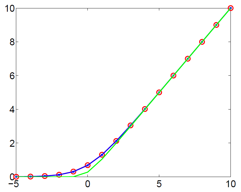
Rectified linear (2)

The result is a softplus function, which can be approximated by rectified linear function $g(x) = \max(x,0)$.
It is like linear with subdued negative response.

Rectified linear (3)

Can rectified linear represents auto-encoding?

Temporal data

The brains capture temporal relations via signal propagation delay in neurons' dendritic trees — the cable theory. The computational model for discrete-time version is k-step Markov chain.
Graham Taylor presents stacked of temporal restricted Boltzmann machines. This yields recurrent neural networks with layer-by-layer training.

Temporal network

Conditional model

The basic building blocks of temporal deep architecture is the conditional model.
We can influence a neural machine with conditional biases;this is like adding biases to individual neurons while training and inference.

Factored conditional model

Using conditional biases with integrate-and-fire neuron model restricts the neuron's expressive power. The real neurons allow some neuro-transmitters to adjust individual synapse directly. (This yields more entries in the conditional output table.)
Graham Taylor presents factored conditional model that utilizes multiplicative neuron model to allow direct parameterization on each connection. This slightly compromises the expressive power from the full conditional table but only adds small number of parameters to be trained.

LSTM

The de facto standard for dealing with temporal data when this presentation was created is Long short-term memory.
LSTM is an apparatus that contains linear information pathways which are controlled by gates.
Gates act as special priors that control information.
The heart of LSTM is to make everything "differentiable".
Originally, it was created to address the problem of gradient loss in long backward propagation, especially through time.